Sometimes, the frame around a matplotlib plot can detract from the information you are trying to convey.  How do you remove the frame, ticks, or axes from a matplotlib plot?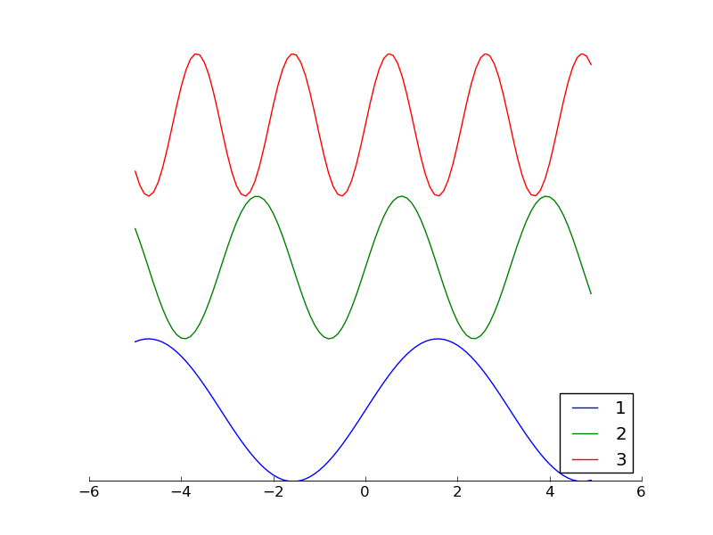

Some books you may find useful when working with matplotlib:

The full example is available on github.

First, we construct a figure and an axes object:

fig1 = plt.figure(facecolor='white')
ax1 = plt.axes(frameon=False)

The Axes object is a container that holds the axes, the ticks, the labels, the plot, the legend, etc.  You will always have an Axes object, even if the axes are not visible! The keyword argument frameon=False turns the frame off. An alternative method is:

In a previous post, I described how Python’s Pickle module is fast and convenient for storing all sorts of data on disk. More recently, I showed how to profile the memory usage of Python code.  In recent weeks, I’ve uncovered a serious limitation in the Pickle module when storing large amounts of data: Pickle requires a large amount of memory to save a data structure to disk. Fortunately, there is an open standard called HDF, which defines a binary file format that is designed to efficiently store large scientific data sets. I will demonstrate both approaches, and profile them to see how much memory is required. I am writing the HDF file using the PyTables interface. Here’s the little test program I’ve been using: [code language=“Python”]#!/usr/bin/env python from numpy import array

I spent some time today profiling a Brownian dynamics simulation written in Python to see how I could make it faster before starting some long runs on a Linux cluster. In the sections below, I have attempted to quantify the speed improvements due to various changes. Keep in mind that the actual speed improvement in your code will vary, depending on where the actual bottlenecks occur. See my post about profiling Python code. Another caveat: I am running Python 2.4.4 because it’s installed on our cluster.

Numerical programming frequently requires the use of look-up tables. A look-up table is a collection of pre-computed values. When given an “x” value, the table returns a pre-computed “y” value. Look-up tables can be used to speed up numerical codes, when it is faster to look up a value in the table than it is to compute the value. They are also used when the data in the table cannot be computed–for example, experimental data or averaged results from an ensemble of Monte Carlo simulations. Another application is to compute a value when a function cannot be solved algebraically. Assume that you have a formula for a function q(h). You need the value of h for a given value of q, but the formula cannot be algebraically solved to get h(q). Instead, choose a range of h values, compute the function q(h), and store each value in a look-up table. Now you can get h(q) for any value stored in the table. The major limitation of a look-up table is that it cannot return valid results for any value of q which is outside the range of those stored in the table. Depending on its implementation, the table may be able to interpolate to return values between known points.

Today I installed numpy on a cluster. Normally, as a Gentoo admin, I just install things with emerge, and all the details are taken care of automagically. However, this cluster runs Red Hat Enterprise, and I don’t have admin privileges, so I had to install numpy in my home directory. I installed 1.0.4, to match the version used on another system. You may not need to do this for more recent versions of numpy, which may have an improved setup script. The overall process is: